30 January 2020

Correlation between mutual fund and index

by Yeung Ka Ming, CFA

Summary

To see how the selected mutual fund performed verse a major China A-share market index.

Mutual fund - AMUNDI INTERINVEST CHINA A SHARES[1]

China A-share market index - CSI300[2]

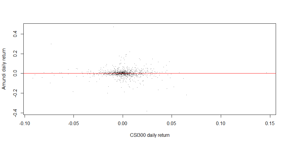
The mutual fund return is negatively correlated to CSI300. One of the reasons might be due to 2015 Chinese Yuan devaluation.
Regression shows that CSI300 cannot explain the performance of the fund. The fund is very likely employing active management.

R Libraries

library("quantmod")
library("tidyverse")
library("tidyquant")
library("PerformanceAnalytics")

Preparation of data

Data is directly downloaded from web, which is publicly available:

data_csi300_tbl <- read_csv("CSI300.csv", col_types = "Dd")
data_amundi_tbl <- read_csv("amundi.csv", col_types = "Dd")

Daily log returns of the fund and the index are calculated:

data_csi300_tbl <- data_csi300_tbl %>% mutate(csi300_return = log(CSI300_Close) - log(lag(CSI300_Close)))
data_amundi_tbl <- data_amundi_tbl %>% mutate(amundi_return = log(amundi) - log(lag(amundi)))

Combine two tibbles by left_join:

data1 <- data_csi300_tbl %>% left_join(data_amundi_tbl, by =c("Date")) %>% drop_na()

Correlation results

Correlation result is listed below:

amundi_csi300 <- cor(data1$csi300_return, data1$amundi_return)

knitr::kable(c(Amundi = amundi_csi300), 
             col.names = "Amundi correlation w/ CSI300")

	Amundi correlation w/ CSI300
Amundi	-0.0323986

Interesting, the fund is negatively correlated with CSI300. The cumulative return of the fund and index are:

csi300_ret <- tail(data1$CSI300_Close,1) / head(data1$CSI300_Close,1)
amundi_ret <- tail(data1$amundi,1) / head(data1$amundi,1)

knitr::kable(c(CSI300 = csi300_ret, Amundi = amundi_ret), 
             col.names = "Cumulative return")

	Cumulative return
CSI300	1.709906
Amundi	1.986001

One of the reasons can be attributed to 2015 Chinese Yuan devaluation. We can also see that from Amundi chart in the website, the performace between the fund and the index diverages starting from 2015.

Regression with CSI300

Daily return regression between the fund and the index is analysed below:

reg1 <- lm(amundi_return ~ csi300_return, data1)

We can tell from the regression result that CSI300 actually cannot explain the return of the fund, so the portfolio manager is very like employing active management.

summary(reg1)

## 
## Call:
## lm(formula = amundi_return ~ csi300_return, data = data1)
## 
## Residuals:
##      Min       1Q   Median       3Q      Max 
## -0.38021 -0.01037 -0.00087  0.00997  0.46852 
## 
## Coefficients:
##                 Estimate Std. Error t value Pr(>|t|)
## (Intercept)    0.0006502  0.0013307   0.489    0.625
## csi300_return -0.0794834  0.0766627  -1.037    0.300
## 
## Residual standard error: 0.04259 on 1023 degrees of freedom
## Multiple R-squared:  0.00105,    Adjusted R-squared:  7.318e-05 
## F-statistic: 1.075 on 1 and 1023 DF,  p-value: 0.3001

plot(data1$csi300_return, data1$amundi_return, pch=".", xlab = "CSI300 daily return", ylab = "Amundi daily return")
abline(lm(data1$csi300_return ~ data1$csi300_return), col='red', lwd=1)

Reference

tags: correlation - regression