Plot Hong Kong Air Pollutants

Summary

Plot Hong Kong Air Pollutants

R Libraries

library(lubridate)
library(ggplot2)
library(tidyverse)

Preparation of data

airpollutants <- read.csv("airpollutants.csv", header = TRUE, sep = ",", encoding ="UTF-8")
head(airpollutants)

##       StationName                        DateTime  NO2   O3 SO2 CO PM10 PM2.5
## 1 Central/Western Thu, 24 Feb 2022 22:00:00 +0800 79.7 35.3 4.5  - 35.7  25.5
## 2 Central/Western Thu, 24 Feb 2022 23:00:00 +0800 98.1 19.1 4.4  - 37.2  25.9
## 3 Central/Western Fri, 25 Feb 2022 00:00:00 +0800 79.0 29.5 3.6  - 35.8  24.9
## 4 Central/Western Fri, 25 Feb 2022 01:00:00 +0800 72.6 29.1 2.7  - 32.4  22.7
## 5 Central/Western Fri, 25 Feb 2022 02:00:00 +0800 36.2 58.9 2.3  - 27.3  20.6
## 6 Central/Western Fri, 25 Feb 2022 03:00:00 +0800 32.5 50.4 2.3  - 24.4  19.2

airpollutants.tbl <- as_tibble(airpollutants)
airpollutants.tbl <- airpollutants.tbl %>% 
  mutate(NO2 = as.double(NO2)) %>% 
  mutate(O3 = as.double(O3)) %>%
  mutate(SO2 = as.double(SO2)) %>% 
  mutate(CO = as.double(CO)) %>% 
  mutate(PM2.5 = as.double(PM2.5))

This part is important for keeping the date and time data

prev <- Sys.getlocale("LC_TIME"); Sys.setlocale("LC_TIME", "C") # help from strptime in R Documentation

## [1] "C"

airpollutants.tbl <- airpollutants.tbl %>% 
  mutate(DateTime = as_datetime(DateTime, format="%a, %d %b %Y %H:%M:%S %z")) # as_datetime from package lubridate

Plot data

airpollutants.long.tbl <- airpollutants.tbl %>% 
  pivot_longer(cols = c(NO2, O3, SO2, CO, PM10, PM2.5), 
               names_to = "pollutants", 
               values_to = "level")

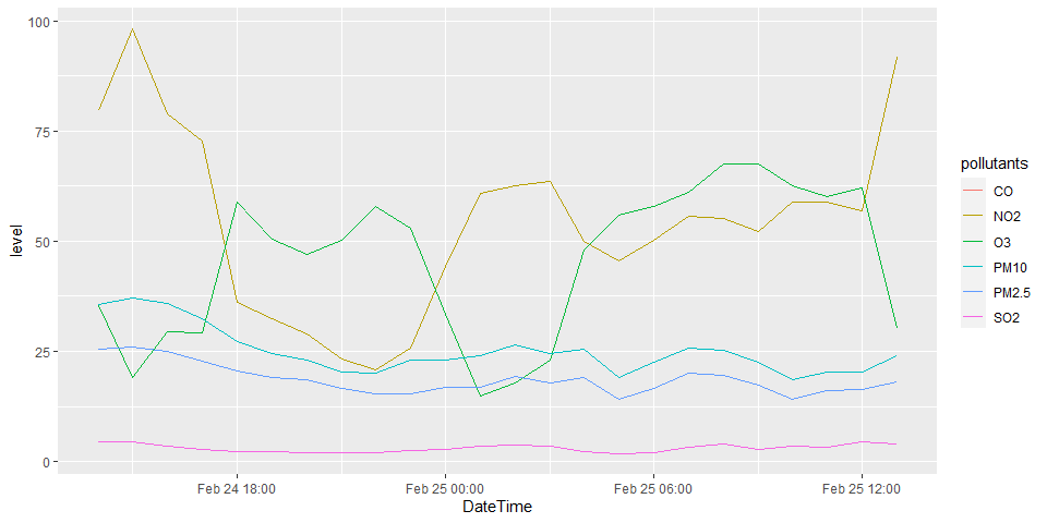
p1 <- airpollutants.long.tbl %>% 
  filter(StationName == "Central/Western") %>% 
  ggplot(aes(x=DateTime, y=level, color=pollutants))
p1 + geom_line()

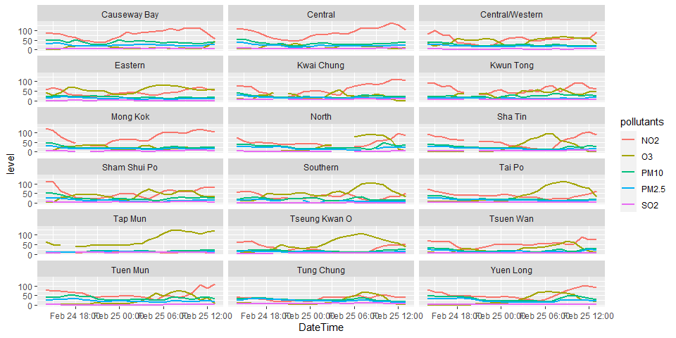
p2 <- airpollutants.long.tbl %>%
  filter(pollutants != "CO") %>% 
  ggplot(aes(x=DateTime, y=level, color=pollutants))
p2 + geom_line(size = 1) + facet_wrap(. ~ StationName, ncol = 3)