iyeung144.github.io
My Github Pages
Hong Kong Stock 2
by Yeung Ka Ming, CFA
Summary
Make a simple portfolio and plot value verse time
R Libraries
library(quantmod)
library(tidyverse)
library(ggplot2)
Preparation of data
Direct download by getSymbols
tickers <- c("0005.HK","9988.HK")
hkport <- new.env()
getSymbols(tickers,
           env=hkport,
           src = "yahoo",
           index.class = "POSIXct",
           from = "2022-01-01")
## [1] "0005.HK" "9988.HK"
# auto.assign is FALSE, so an environment is used here. Unlike US stocks,
# the tickers in HK stock market is by number, which cannot be the variable
# name in R. Further fine tune in next step
Rename column names
HSBC<-hkport$`0005.HK`
BABA<-hkport$`9988.HK`

# substitute numeric ticker name to character name. It is inconvenient to handle
# variable name starts with number.
colnames(BABA) <- sub("9988.HK","BABA",colnames(hkport$`9988.HK`))
head(hkport$`9988.HK`)
##            9988.HK.Open 9988.HK.High 9988.HK.Low 9988.HK.Close 9988.HK.Volume 9988.HK.Adjusted
## 2022-01-03        117.0        117.5       114.0         115.0       22176946            115.0
## 2022-01-04        118.4        118.9       115.7         116.9       23228903            116.9
## 2022-01-05        119.0        119.1       113.9         114.5       30717509            114.5
## 2022-01-06        117.5        121.1       117.3         121.0       47231895            121.0
## 2022-01-07        126.5        128.8       122.8         128.8       58778943            128.8
## 2022-01-10        128.8        129.5       125.4         127.6       36814976            127.6
head(BABA)
##            BABA.Open BABA.High BABA.Low BABA.Close BABA.Volume BABA.Adjusted
## 2022-01-03     117.0     117.5    114.0      115.0    22176946         115.0
## 2022-01-04     118.4     118.9    115.7      116.9    23228903         116.9
## 2022-01-05     119.0     119.1    113.9      114.5    30717509         114.5
## 2022-01-06     117.5     121.1    117.3      121.0    47231895         121.0
## 2022-01-07     126.5     128.8    122.8      128.8    58778943         128.8
## 2022-01-10     128.8     129.5    125.4      127.6    36814976         127.6
colnames(HSBC) <- sub("0005.HK","HSBC",colnames(hkport$`0005.HK`))
head(hkport$`0005.HK`)
##            0005.HK.Open 0005.HK.High 0005.HK.Low 0005.HK.Close 0005.HK.Volume 0005.HK.Adjusted
## 2022-01-03        47.00        47.15       46.65         46.85        6711558            46.85
## 2022-01-04        47.10        47.80       47.00         47.80       25500155            47.80
## 2022-01-05        49.35        49.75       48.75         49.15       59292303            49.15
## 2022-01-06        49.05        49.05       48.35         49.00       24559582            49.00
## 2022-01-07        50.10        50.15       49.75         50.10       67407695            50.10
## 2022-01-10        50.80        51.75       50.60         51.70       59640904            51.70
head(HSBC)
##            HSBC.Open HSBC.High HSBC.Low HSBC.Close HSBC.Volume HSBC.Adjusted
## 2022-01-03     47.00     47.15    46.65      46.85     6711558         46.85
## 2022-01-04     47.10     47.80    47.00      47.80    25500155         47.80
## 2022-01-05     49.35     49.75    48.75      49.15    59292303         49.15
## 2022-01-06     49.05     49.05    48.35      49.00    24559582         49.00
## 2022-01-07     50.10     50.15    49.75      50.10    67407695         50.10
## 2022-01-10     50.80     51.75    50.60      51.70    59640904         51.70
Prepare a dataframe with portfolio value and plot graph
Prepare dataframe
# Suppose $100,000 for investment on the first trading day of 2022.
# Use around half of the amount for each stock

moneyseed <- 100000
portion <- 0.5
shares <- c(portion*moneyseed/HSBC$HSBC.Adjusted[[1]],portion*moneyseed/BABA$BABA.Adjusted[[1]])

# need stock adjusted prices and number of shares to make a portfolio
prices.tbl <- as_tibble(fortify(merge(HSBC, BABA)))

port.tbl <- prices.tbl %>% select(Index,HSBC.Adjusted,BABA.Adjusted)
port.tbl
## # A tibble: 42 x 3
##    Index               HSBC.Adjusted BABA.Adjusted
##    <dttm>                      <dbl>         <dbl>
##  1 2022-01-03 00:00:00          46.8          115
##  2 2022-01-04 00:00:00          47.8          117.
##  3 2022-01-05 00:00:00          49.2          114.
##  4 2022-01-06 00:00:00          49            121
##  5 2022-01-07 00:00:00          50.1          129.
##  6 2022-01-10 00:00:00          51.7          128.
##  7 2022-01-11 00:00:00          52.0          126.
##  8 2022-01-12 00:00:00          52.8          133
##  9 2022-01-13 00:00:00          53.7          132.
## 10 2022-01-14 00:00:00          54.5          129.
## # ... with 32 more rows
port.tbl <- port.tbl %>% mutate(port.value = shares[1]*HSBC.Adjusted+shares[2]*BABA.Adjusted)
port.tbl
## # A tibble: 42 x 4
##    Index               HSBC.Adjusted BABA.Adjusted port.value
##    <dttm>                      <dbl>         <dbl>      <dbl>
##  1 2022-01-03 00:00:00          46.8          115     100000
##  2 2022-01-04 00:00:00          47.8          117.    101840.
##  3 2022-01-05 00:00:00          49.2          114.    102237.
##  4 2022-01-06 00:00:00          49            121     104903.
##  5 2022-01-07 00:00:00          50.1          129.    109469.
##  6 2022-01-10 00:00:00          51.7          128.    110654.
##  7 2022-01-11 00:00:00          52.0          126.    110052.
##  8 2022-01-12 00:00:00          52.8          133     114123.
##  9 2022-01-13 00:00:00          53.7          132.    114735.
## 10 2022-01-14 00:00:00          54.5          129.    114435.
## # ... with 32 more rows
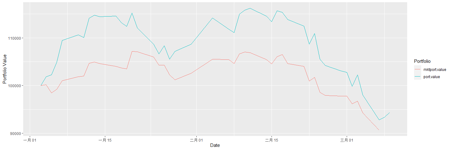
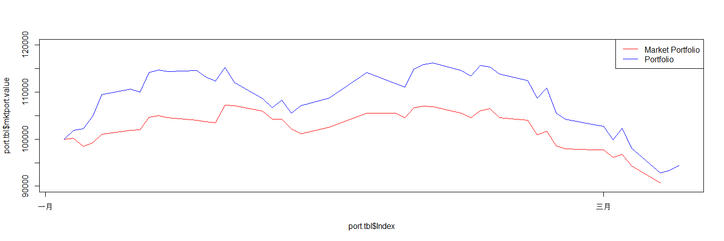
Plot graph
plot(x=port.tbl$Index,y=port.tbl$port.value, type="l")
p1 <- ggplot(port.tbl, aes(x=Index,y=port.value))
p1 + xlab("Date") + ylab("Portfolio Value") + geom_line()