Hong Kong Stock 5

Summary

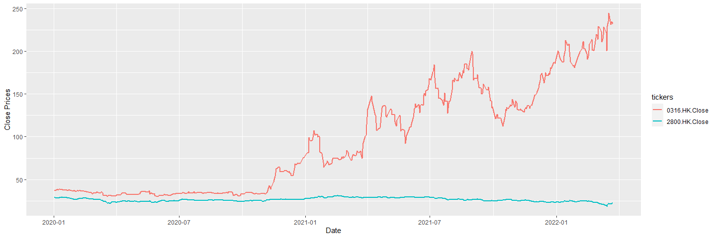
OOCL is a shipping company and the performance during the pandemic is extraordinary.

R Libraries

library(quantmod)
library(tidyverse)
library(ggplot2)

Preparation of data

Direct download by getSymbols

tickers <- c('0316.HK','2800.HK')
hkport <- new.env()
getSymbols(tickers, 
           env=hkport, 
           src = "yahoo",
           index.class = "POSIXct",
           from = "2020-01-01")

## [1] "0316.HK" "2800.HK"

# auto.assign is FALSE, so an environment is used here. 
# Unlike US stocks, # the tickers in HK stock market is 
# by number, which cannot be the variable
# name in R. Further fine tune in next step.

OHLC price

head(Ad(hkport$`0316.HK`))

##            0316.HK.Adjusted
## 2020-01-02         29.70684
## 2020-01-03         29.15525
## 2020-01-06         30.61301
## 2020-01-07         29.94323
## 2020-01-08         29.78563
## 2020-01-09         30.88880

head(Cl(hkport$`0316.HK`))

##            0316.HK.Close
## 2020-01-02         37.70
## 2020-01-03         37.00
## 2020-01-06         38.85
## 2020-01-07         38.00
## 2020-01-08         37.80
## 2020-01-09         39.20

head(Op(hkport$`0316.HK`))

##            0316.HK.Open
## 2020-01-02        37.80
## 2020-01-03        37.65
## 2020-01-06        37.05
## 2020-01-07        37.65
## 2020-01-08        37.65
## 2020-01-09        38.45

head(Hi(hkport$`0316.HK`))

##            0316.HK.High
## 2020-01-02        37.80
## 2020-01-03        37.80
## 2020-01-06        39.45
## 2020-01-07        38.75
## 2020-01-08        39.35
## 2020-01-09        39.20

head(Lo(hkport$`0316.HK`))

##            0316.HK.Low
## 2020-01-02       37.75
## 2020-01-03       37.00
## 2020-01-06       37.05
## 2020-01-07       37.65
## 2020-01-08       37.65
## 2020-01-09       37.60

Prepare a dataframe with all adjusted close prices

Prepare dataframe

## To get all the close prices
## into a single xts object
cl.stocks.xts <- Reduce(merge,eapply(hkport, Cl))
colnames(cl.stocks.xts) <- sub('X','',colnames(cl.stocks.xts))

cl.stocks.tbl <- as_tibble(fortify(cl.stocks.xts))
cl.stocks.long.tbl <- cl.stocks.tbl %>% 
  pivot_longer(!Index,
               names_to = "tickers", 
               values_to = "Close.Prices")
cl.stocks.long.tbl

## # A tibble: 1,102 x 3
##    Index               tickers       Close.Prices
##    <dttm>              <chr>                <dbl>
##  1 2020-01-02 00:00:00 0316.HK.Close         37.7
##  2 2020-01-02 00:00:00 2800.HK.Close         28.7
##  3 2020-01-03 00:00:00 0316.HK.Close         37  
##  4 2020-01-03 00:00:00 2800.HK.Close         28.6
##  5 2020-01-06 00:00:00 0316.HK.Close         38.8
##  6 2020-01-06 00:00:00 2800.HK.Close         28.5
##  7 2020-01-07 00:00:00 0316.HK.Close         38  
##  8 2020-01-07 00:00:00 2800.HK.Close         28.5
##  9 2020-01-08 00:00:00 0316.HK.Close         37.8
## 10 2020-01-08 00:00:00 2800.HK.Close         28.2
## # ... with 1,092 more rows

Plot graph

p4 <- ggplot(cl.stocks.long.tbl,
            aes(x = Index, 
                y = Close.Prices,
                color=tickers))
p4 + 
  geom_line(size = 1) + 
  xlab("Date") + 
  ylab("Close Prices")